Fedora 19

⁠Amateur Radio Guide

A guide for users of Fedora amateur radio software

The Fedora Documentation Project

Legal Notice

The text of and illustrations in this document are licensed by Red Hat under a Creative Commons Attribution–Share Alike 3.0 Unported license ("CC-BY-SA"). An explanation of CC-BY-SA is available at http://creativecommons.org/licenses/by-sa/3.0/. The original authors of this document, and Red Hat, designate the Fedora Project as the "Attribution Party" for purposes of CC-BY-SA. In accordance with CC-BY-SA, if you distribute this document or an adaptation of it, you must provide the URL for the original version.

Red Hat, as the licensor of this document, waives the right to enforce, and agrees not to assert, Section 4d of CC-BY-SA to the fullest extent permitted by applicable law.

Red Hat, Red Hat Enterprise Linux, the Shadowman logo, JBoss, MetaMatrix, Fedora, the Infinity Logo, and RHCE are trademarks of Red Hat, Inc., registered in the United States and other countries.

For guidelines on the permitted uses of the Fedora trademarks, refer to https://fedoraproject.org/wiki/Legal:Trademark_guidelines.

Linux® is the registered trademark of Linus Torvalds in the United States and other countries.

Java® is a registered trademark of Oracle and/or its affiliates.

XFS® is a trademark of Silicon Graphics International Corp. or its subsidiaries in the United States and/or other countries.

MySQL® is a registered trademark of MySQL AB in the United States, the European Union and other countries.

All other trademarks are the property of their respective owners.

Abstract

Fedora includes a wide range of applications relevant to amateur radio operators. This guide describes the use of some of those applications.

⁠1. Introduction

Amateur radio and Linux go hand-in-hand. Both allow users to experiment to the extent of their knowledge and to learn more along the way. With new digital technologies being used everyday open source software is the best way to stay cutting edge in this ever-changing hobby.

Fedora has packaged dozens of software to make it easy for Fedora users to obtain and setup. Within seconds any user will be able to have the tools they to enhance their amateur radio experience.

⁠2. Sound Card Modes

This section describes the sound card modes.

⁠2.1. fldigi

fldigi is one of the most robust soundcard modem software around. It supports CW, DominioEX, Feld-Hell, MFSK, MT-63 PSK, OLIVIA, RTTY, Thor, and Throb. fldigi also includes, as part of the software, a logger which is smart enough to almost complete itself.

⁠

Figure 1. fldigi

⁠3. Rig Control

This section describes rig control applications.

⁠3.1. Chirp

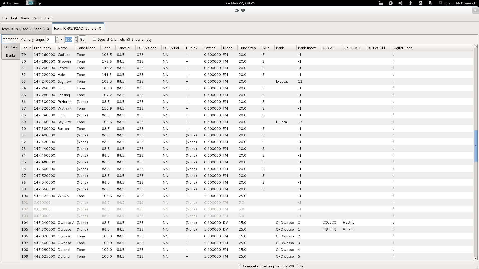
chirp is an application that allows programming of radios from a number of vendors. Chirp assumes that the appropriate cable is available and connected. Data may be saved to a .csv file for manipulation by other applications, as well as transferred between radios, even radios from different manufacturers.

chirp is started by clicking the chirp icon.

⁠

Figure 2. Chirp icon

This will present a rather uninteresting blank screen.

In most cases, the user will wish to begin by selecting Download from Radio from the Radio menu. This will launch a dialog requesting some basic information such as the desired serial port, radio vendor and model. Note that the selected serial port must permit read/write access.

⁠

Figure 3. Chirp Radio Dialog

Clicking the OK button will begin reading the radio's memory.

What happens next depends on the radio. For radios that operate in "live" mode, the values will appear in the window, and values at the bottom of the window will show how many memories remain to be read and how many have been read. For radios with multiple bands, the first value will alternate between bands.

⁠

Figure 4. Chirp Main Screen

For radios that do not operate in "live" mode, a small window containing a progress bar will show the progress of the download. The data will appear after the data has been downloaded.

⁠

Figure 5. Chirp Main Screen

To change a value, simply click on the field and begin typing.

⁠

Figure 6. Changing a memory location

On some radios, data is changed in the radio as soon as it is changed onscreen. For others, it will be necessary to select the Upload to Radio from the Radio menu.

⁠

Figure 7. Chirp Main Screen

A progress bar will be displayed similar to that displayed during data download.

⁠

Figure 8. Chirp Main Screen

By default, only the first 25 memories are displayed. Near the top of the screen the Memory range controls allow for selecting those memories to be displayed. If a large number of memories are selected, it may take some time to display.

⁠

Figure 9. Selecting Memory Range to Display

Depending on the radio, there may be quite a few columns to display, so maximizing the window could be helpful.

⁠

Figure 10. Large Display

Individual columns may be removed from the display, making the display more manageable.

⁠

Figure 11. Selecting Columns

⁠3.2. grig

grig is a simple front panel for a radio.

To start grig, click the grig icon:

⁠

Figure 12. grig icon

When started from the menu, grig uses a dummy back end, so you may explore the capability, but your radio will not be affected.

The main window allows for control over most of the actions accessible from a typical radio front panel. Frequency may be increased or decreased by left or right clicking the appropriate digit in the frequency display. Other controls are more or less self-explanatory.

⁠

Figure 13. grig main window

To control the radio, you should start grig from the command line. You must first have your radio connected using the appropriate hardware, which most commonly will be a serial port.

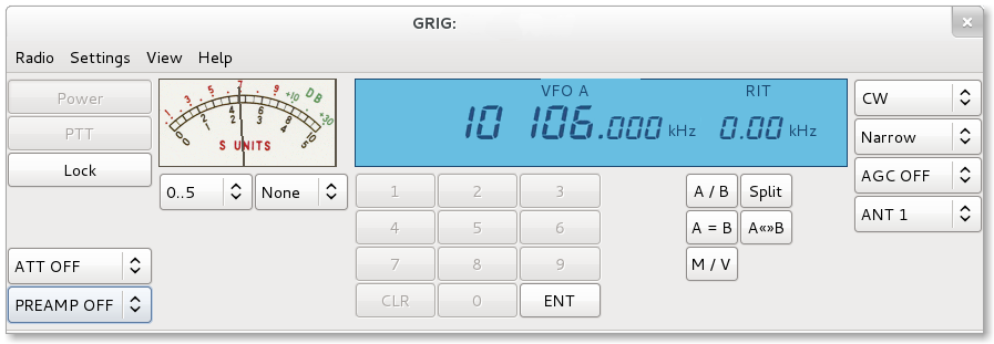
You must provide grig with the model code for your radio, the port and speed, and in some cases, a radio address. You can find the model code by typing rigctl -l. Use man grig or info grig for all the possible switches, but most commonly you will use -m for the model, -r for the port, -s for the speed, and most often, -c for the address.

For example, for an Icom 7000 on /dev/ttyUSB0, the command would be:

grig -m 360 -r /dev/ttyUSB0 -s 9600 -c 0x70

The -m 360 is the model code for an Icom 7000, the -r /dev/ttyUSB0 is the port to which the radio is attached, the -s 9600 is the baud rate, and -c 0x70 is the default CIV address for an Icom 7000.

Since you typically will have only a few radios, it may be preferable to create a script, or perhaps edit /usr/share/applications/fedora-grig.desktop to reflect your particular hardware.

⁠3.3. hamlib

hamlib is a library to be used by other programs to interface to radios and rotors. However, since hamlib maintains no configuration information (type of rig, connection method, etc.) itself, programs must provide that configuration.

Some programs such as fldigi provide the necessary hamlib information in a fashion somewhat hidden from the user, but others (grig, soundmodem) require the user understand hamlib configuration. Even with fldigi, advanced users may find it necessary to provide hamlib commands.

While primarily for use with other programs, hamlib includes a few applications which may be used directly, including:

rigctl - allows for control of the rig from the command line
rigmem - save and restore a radio's memories
rigswr - measure SWR across a range of frequencies
rotctl - control the rotor
rigsmtr - collect S meter readings versus azimuth. Needs rotctl.

In addition, there are daemons provided for controlling the rig and rotor.

The various hamlib applications require certain switches to describe the rig and its connection, and most take a number of commands.

⁠

Table 1. Rig description switches

Switch	Meaning
`-m, --model=id`	Select radio model number. See model list (use '`rigctl -l`').
`-r, --rig-file=device`	Use device as the file name of the port the radio is connected. Often a serial port, but could be a USB to serial adapter. Typically `/dev/ttyS0`, `/dev/ttyS1`, `/dev/ttyUSB0`, etc.
`-p, --ptt-file=device`	Use device as the file name of the Push-To-Talk device using a device file as described above.
`-d, --dcd-file=device`	Use device as the file name of the Data Carrier Detect device using a device file as described above.
`-P, --ptt-type=type`	Use type of Push-To-Talk device. Supported types are RIG, DTR, RTS, PARALLEL, NONE, overriding PTT type defined in the rig's backend.
`-D, --dcd-type=type`	Use type of Data Carrier Detect device. Supported types are RIG, DSR, CTS, CD, PARALLEL, NONE.
`-s, --serial-speed=baud`	Set serial speed to baud rate. Uses maximum serial speed from rig backend capabilities as the default.
`-c, --civaddr=id`	Use id as the CI-V address to communicate with the rig. Only useful for Icom rigs.
`-t, --send-cmd-term=char`	Change the termination char for text protocol when using the send_cmd command. The default value is <CR> (0x0d). Non ASCII printable characters can be specified as an ASCII number, in hexadecimal format, prepended with 0x. You may pass an empty string for no termination char. The string '`-1`' tells rigctl to switch to binary protocol. See the send_cmd command for further explanation.
`-L, --show-conf`	List all config parameters for the radio defined with `-m` above.
`-C, --set-conf=parm=val[,parm=val]`	Set config parameter. e.g. `stop_bits=2`. Use `-L` option for a list.
`-l, --list`	List all model numbers defined in Hamlib and exit.
`-u, --dump-caps`	Dump capabilities for the radio defined with `-m` above and exit.
`-o, --vfo`	Set vfo mode, requiring an extra VFO argument in front of each appropriate command. Otherwise, VFO_CURR is assumed when this option is not set.
`-v, --verbose`	Set verbose mode, cumulative.
`-h, --help`	Show summary of these options and exit.
`-V, --version`	Show version of rigctl and exit.

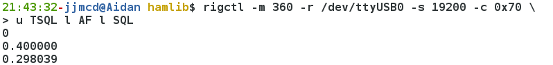
For example, to communicate with an Icom 7000 on /dev/ttyUSB0 at 19,200 baud:

      rigctl -m 360 -r /dev/ttyUSB0 -s 19200 -c 0x70

⁠3.3.1. rigctl

rigtcl can accept a large number of commands, either on the command line or in interactive mode. The following table lists some of the more common commands. For more details see man rigctl.

⁠

Table 2. Rig description switches

Command	Meaning
`F, set_freq 'Frequency'`	Set 'Frequency', in Hz.
`f, get_freq`	Get 'Frequency', in Hz.
`M, set_mode 'Mode' 'Passband'`	Set 'Mode': USB, LSB, CW, CWR, RTTY, RTTYR, AM, FM, WFM, AMS, PKTLSB, PKTUSB, PKTFM, ECSSUSB, ECSSLSB, FAX, SAM, SAL, SAH, DSB.
`m, get_mode`	Get 'Mode' 'Passband'.
`V, set_vfo 'VFO'`	Set 'VFO': VFOA, VFOB, VFOC, currVFO, VFO, MEM, Main, Sub, TX, RX.
`v, get_vfo`	Get current 'VFO'.
`R, set_rptr_shift 'Rptr Shift'`	Set 'Rptr Shift': "+", "-" or something else for none.
`r, get_rptr_shift`	Get 'Rptr Shift'. Returns "+", "-" or "None".
`O, set_rptr_offs 'Rptr Offset'`	Set 'Rptr Offset', in Hz.
`o, get_rptr_offs`	Get 'Rptr Offset', in Hz.
`U, set_func 'Func' 'Func Status'`	Set 'Func' 'Func Status'. Func is one of: FAGC, NB, COMP, VOX, TONE, TSQL, SBKIN, FBKIN, ANF, NR, AIP, APF, MON, MN, RF, ARO, LOCK, MUTE, VSC, REV, SQL, ABM, BC, MBC, AFC, SATMODE, SCOPE, RESUME, TBURST, TUNER.
`u, get_func`	Get 'Func' 'Func Status'.
`L, set_level 'Level' 'Level Value'`	Set 'Level' and 'Level Value'. Level is one of: PREAMP, ATT, VOX, AF, RF, SQL, IF, APF, NR, PBT_IN, PBT_OUT, CWPITCH, RFPOWER, MICGAIN, KEYSPD, NOTCHF, COMP, AGC (0:OFF, 1:SUPERFAST, 2:FAST, 3:SLOW, 4:USER, 5:MEDIUM, 6:AUTO), BKINDL, BAL, METER, VOXGAIN, ANTIVOX, SLOPE_LOW, SLOPE_HIGH, RAWSTR, SWR, ALC, STRENGTH. The Level Value can be a float or an integer.
`l, get_level`	Get 'Level' 'Level Value'. Returns Level as a string from set_level above and Level value as a float or integer.

For example, the following command asks to display the frequency and mode. The mode display always also shows the bandwidth:

⁠

Figure 14. rigctl - show mode and frequency

The following example asks whether the tone squelch is on and what are the volume and squelch control settings:

⁠

Figure 15. rigctl - show tone squelch, AF and Squelch controls

The radio can be controlled as well. In the following example the radio is set to CW mode with a 500 Hz filter, and the frequency is set to 3.563 MHz:

⁠

Figure 16. rigctl - set frequency and mode

⁠3.3.2. rigmem

rigmem reads or restores the radio's memories. rigmem uses the same communication parameters as rigctl folowed by two more parameters; the action to be performed and the file name to save memories to or restore memories from.

rigmem queries the radio for the number of memories available, then asks for all the information about each of those memories. Because not all radios support all possible parameters, this may result in hundreds of messages asrigmem asks the radio questions it cannot answer. These messages are benign.

⁠3.3.3. rigswr

rigswr takes the same communication parameters as the other commands, followed by start and end frequencies and a step size. rigswr then cycles through the frequencies, keying the transmitter in CW mode for a half second at quarter power at each frequency and reporting the SWR. For this to work the rig must support sending the SWR while the rig is keyed.

⁠

Figure 17. rigswr

⁠3.3.4. rotctl

⁠3.3.5. rigsmtr

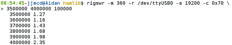
rigsmtr works with rotctl to measure the signal strength versus azimuth. rigsmtr requires both rig and rotor configuration as well as an optional time step. rigsmtr records the S reading every second as the rotor rotates, or every time_step if time_step has been specified. Refer to man rigsmtr.

⁠4. Logging and related applications

⁠4.1. CQRLOG

The CQRLOG program is a great, full-featured, contact log for amateur radio operators. Not only does it maintain your contacts but keeps track of your progress towards common awards including DXCC, WAS, WAC, IOTA, and others. CQRLOG also integrates with DXCluster and fldigi for even more integrated operation in your shack.

CQRLOG also integrates with the ARRL's LoTW (using TrustedQSL), eQSL, Hamlog, Clublog, and other web-based log managers.

⁠4.1.1. Installing CQRLOG

cqrlog is simply installed like most applications:

sudo yum install cqrlog

⁠4.1.2. Starting cqrlog

cqrlog may be started from the menu by selecting Applications->Other->cqrlog or from the command line by typing cqrlog.

⁠4.1.3. Setting up cqrlog

CQRLOG is extremely easy to get setup. The first time you launch the software a database will be created for you. Additional databases may be created for other uses including DXpeditions, other hams, and other purposes as you see fit.

Exception

The first time you start CQRLOG you may experience an exception that will make the software display odd characters. Simply restart the software and all should appear correctly.

After starting CQRLOG, select Home->Preferences to configure all of the software's options.

Additional information on this software, including support, is available at http://cqrlog.com/.

⁠4.2. qle

qle stands for QSO Logger and Editor. It is a simple yet flexible logging program. qle uses a lightweight sqlite database that can be manipulated using standard tools. The application is easily customized, so you can have the logging program behave the way you want. It also interfaces with hamlib, so information may be automatically retrieved from your rig with the appropriate hardware.

⁠4.2.1. Installing qle

qle can be installed with yum like any other package:

sudo yum install qle

However, qle requires some initial setup before it may be used.

⁠4.2.2. Configuring qle

The install process creates a configuration file /etc/qle/qle.conf which must be edited. This can be done with your favorite text editor, however, the file is protected against writing by a non-admin user. The file might be edited with something like:

sudo gedit /etc/qle/qle.conf &

There are two lines that must be changed. At line 63 of the file, you will find the lines:

#
debug = 0
#
myCall = N0CAL
#

Be sure that the debug line is set to zero and change the myCall line to reflect your callsign.

The second line that must be changed is at line 75 where you will find:

# Filename of SQLite DB with full path.
# This file requires sufficient RW access for the DB to work...
#
db = foo3.db
#
# Name of the table that you want to log into.
# Is probably case-sensitive:
#
tableName = mycall
#

You must change the name of the database to your desired name and location.

qle is set up for a single user system, so all users share the same database. You must place the database in a location where it can be accessed by any users requiring it. If you always log on with the same usercode, you might choose to put it in a hidden subdirectory off your logon directory, for example, ~/.qle. This is the simplest approach, but in some circumstances, you may prefer a more "global" location, for example, /etc/qle. In this case, you need to take care to give the file appropriate protections.

For simplicity, we will assume that qle will only ever be run from a single usercode and we will put the database there. Reflect that location and name in qle.conf, for example:

db = /home/usercode/.qle/qle.sqlite

Note that you cannot use the tilde (~) within the config file, you must enter the entire path.

There are many things you may wish to change. For example, at line 101:

#
useRig = 1
#

determines whether you want to use the rig control library, hamlib, which can be a great convenience if you have the appropriate hardware.

At line 225:

#
noCwDaemon = 0
#

determines whether you wish qle to have the capability of keying the transmitter.

To avoid describing hamlib settings and hardware setup, we will assume these are both disabled for now, that is, useRig=0 and noCwDaemon=1.

After editing qle.conf, you need to create the database. There is a sample database in /usr/share/qle so we can copy that to the location we have specified for our database:

cp /usr/share/qle/foo3.db ~/.qle/qle.sqlite

This file has some test data which we will delete after some initial testing.

⁠4.2.3. Running qle for the first time

The first time you run qle, it should be done from the command line in debug mode to be sure you made no errors in the config file:

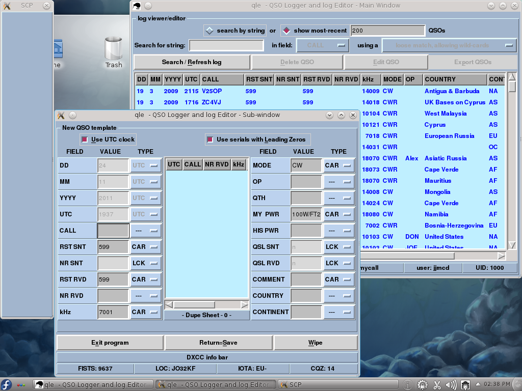
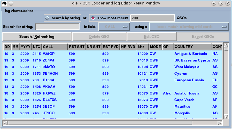
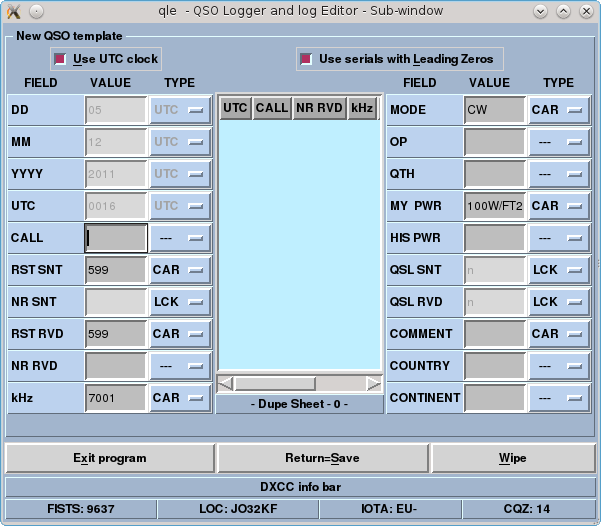
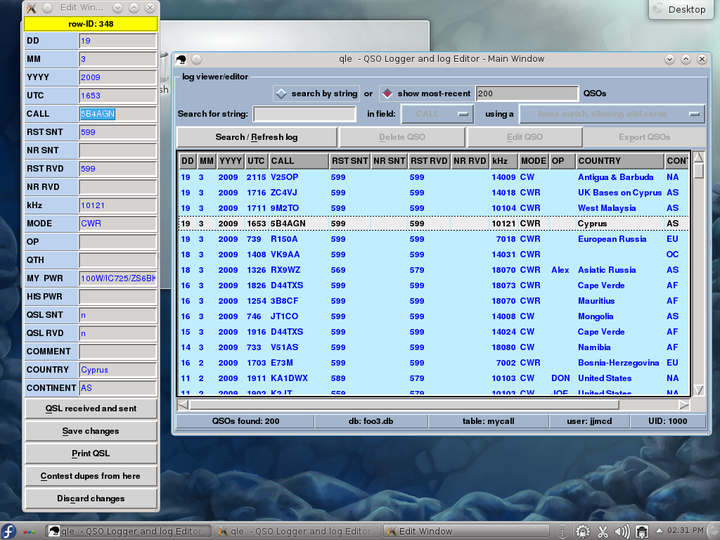
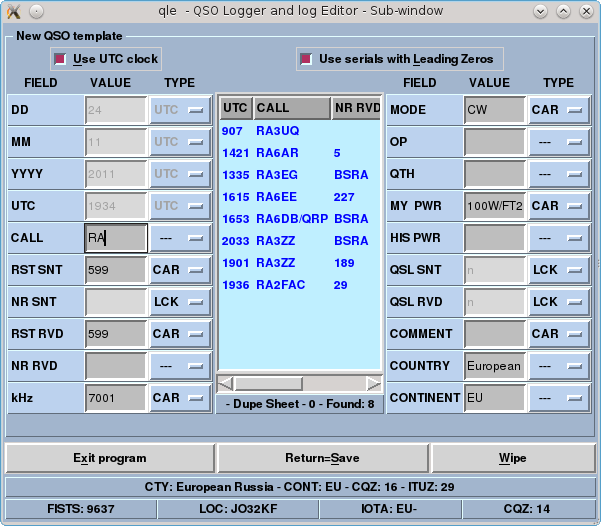
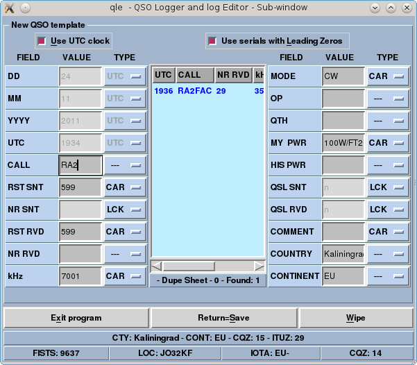
qle --debug=1

If there were errors editing the configuration file, they will appear in the window from which you started qle. If all went well, this should result in seeing the logging windows with the test data displayed:

⁠

Figure 18. Running qle the first time

The qle "Main Window" shows the QSOs that have been logged so far. It will contain QSOs from the sample database. We will delete those QSOs later.

⁠

Figure 19. qle Main Window

The "Sub-Window" is actually where the data will be entered for each QSO. Some fields are provided automatically, such as the date and time. These will be a lighter color than the other fields. Each field has a button to the right indicating how that field is to be treated. Fields that have the label CAR will be carried over from QSO to QSO. These can be overwritten, but will initially be filled in with data from the previous QSO. These are things like Mode, Power, etc that tend not to change.

⁠

Figure 20. qle Data Entry Window

If you wish to change the data in a field that has the label LCK, you may simply click on LCK and select another choice from the dropdown. Normally, you might choose --, but if you are contesting, the NR SENT field includes a +1 choice.`

⁠

Figure 21. Changing Field Attributes

If you double-click an existing QSO in the Main Window, an Editing Window will appear, allowing you to make changes to the existing QSO.

⁠

Figure 22. Editing an existing QSO

To exit the program, click the Exit Program button at the lower left of the subwindow.

⁠

Figure 23. Exit Program Button

qle will ask for confirmation when exiting.

⁠4.2.4. Deleting Sample Data

Now that you are familiar with the basic operation of qle, you will want to delete the original sample data so the database only contains your QSOs. Since the data is in a sqlite database, we merely need to use some simple commands to do that:

[jjmcd@Aidan .qle]$ sqlite3 ~/.qle/qle.sqlite
SQLite version 3.6.20
Enter ".help" for instructions
Enter SQL statements terminated with a ";"
sqlite> DELETE FROM mycall;
sqlite> .quit
[jjmcd@Aidan .qle]$

If you are familiar with SQL, you can also use sqlite to make other changes and queries.

You are now ready to begin using qle. Click on the qle icon, typically found in the "Internet" group.

⁠

Figure 24. qle icon

⁠4.2.5. Duplicate Checking

qle provides duplicate checking as the call is entered. When the first character is entered, any calls in the log that match are shown in the duplicate window:

⁠

Figure 25. Dupe Sheet - first character

As additional characters are entered, the list gets shorter:

⁠

Figure 26. Dupe Sheet - second character

⁠

Figure 27. Dupe Sheet - third character

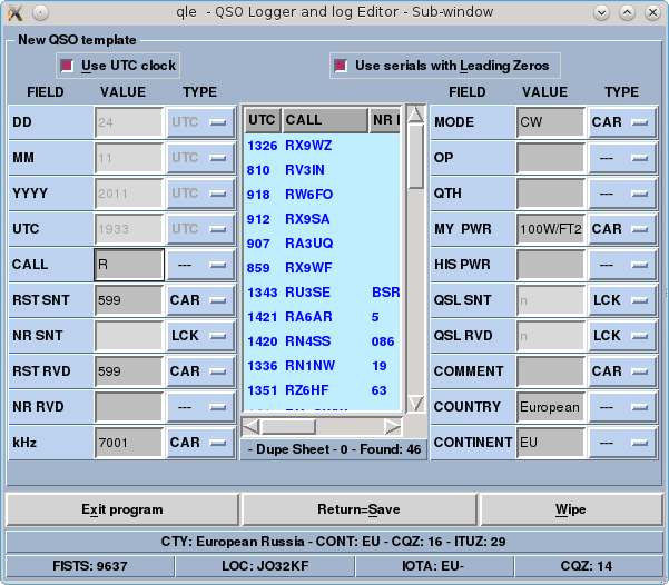
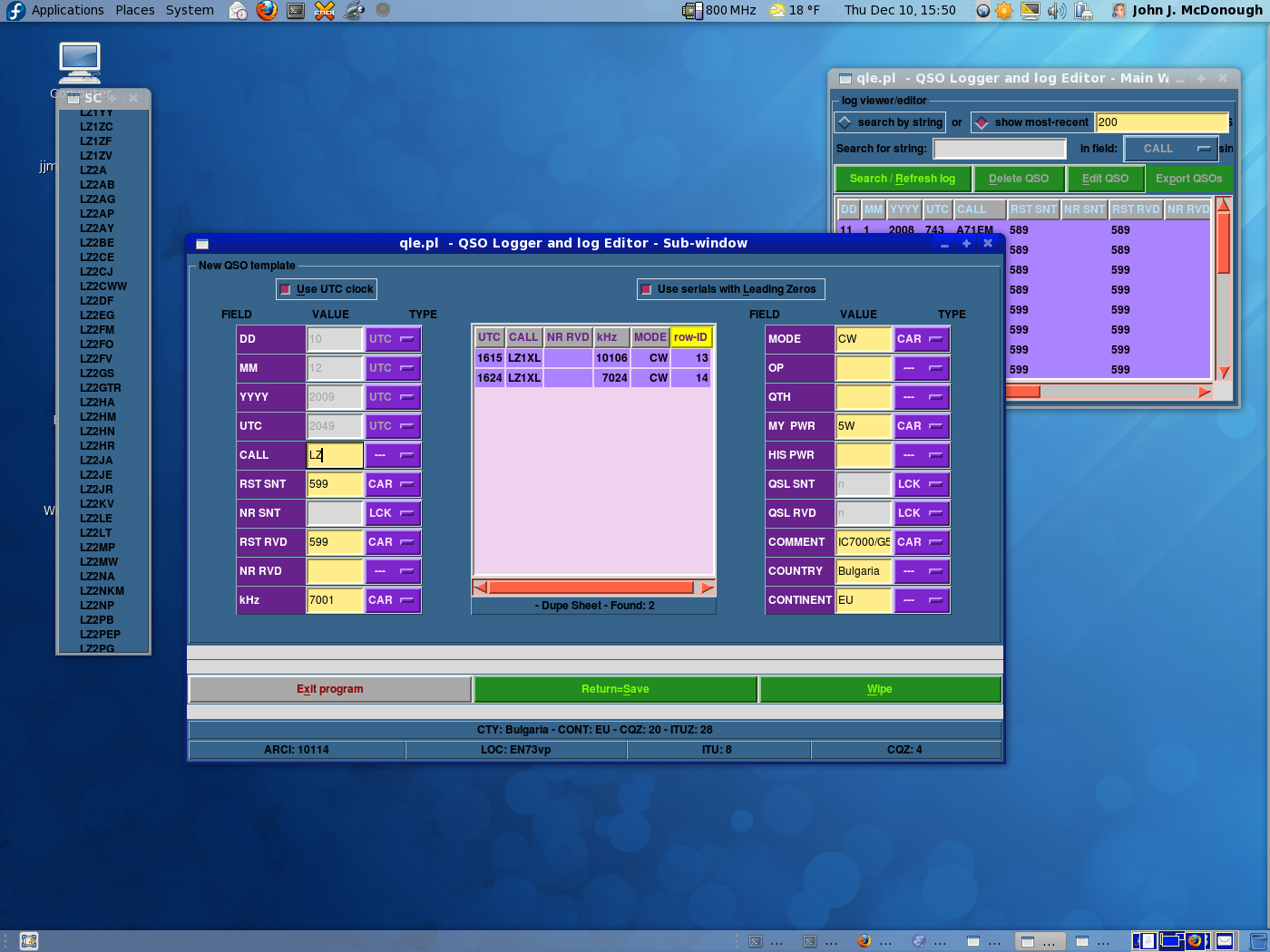
In addition to the current log, the file /usr/share/qle/master.scp contains a list of calls to check. These are shown in a separate SCP window:

⁠

Figure 28. SCP Window

Like the dupes window, this list gets shorter as you type. Edit master.scp to include the calls you want.

⁠4.2.6. Some customizations you probably want

qle is highly customizable. In the previous sections, we described a few things that definitely need to be changed. There are quite a few more you probably want to change.

At the bottom of the secondary screen you will notice a bar with some information:

⁠

Figure 29. Subwindow Info Bar

This bar is simply a reminder for some random data you may want to keep handy. You can change the information by editing the lines starting at line 1051 in the configuration file:

infoString = "ARCI: 10114"
infoString = "LOC: EN73vp"
infoString = "ITU: 8 "
infoString = "CQZ: 4 "

You may find that you want the default field types to be different. For example, suppose you constantly change power and you don't want the previous power to be shown by default. At line 384 of the configuration file is a line for each field with the default type. You can simply change this to make qle start with the type you desire:

fieldTypes =		"---"            # mypwr

You can even adjust individual colors to make them as appealing (or as horrible) as you prefer:

⁠

Figure 30. Colors only a mother could love

There are literally hundreds of adjustments you can make to tailor your logger to behave exactly the way you want. Just be sure to carefully review the comments in qle.conf so you don't get unexpected results.

⁠4.3. xlog

xlog is a wonderful logging program that allows the user to create multiple logs, import and export in various formats, and maintain a count on the various awards such as WAS, WAC, DXCC, WAZ, and IOTA. Future versions will contain code to hook into the ARRL's LoTW.

⁠4.3.1. Installing xlog

xlog is simply installed like most applications:

sudo yum install xlog

⁠4.3.2. Starting xlog

xlog may be started from the menu by selecting Applications->Other->xlog or from the command line by typing xlog.

⁠4.3.3. Setting up xlog

xlog is extremely easy to get setup. After starting xlog, select Settings->Preferences. This will bring up a preferences box where you can configure most options for xlog.

The General tab contains basic information on how the log will be setup including the modes and bands you operate. You can change these at anytime but it is good to go ahead and add or remove the modes and bands you don't operate to simplify the operation of the logging later. You can also enable the clock on the status bar and recording of azimuth and distance when you enter in the location of the station. You can also control out data from external programs, such as gmfsk and ktrack, are handled.

The Info tab contains information on your station and preference to miles or kilometers and where you want the software to look up a callsign. It is recommended that you enter your callsign and your coordinates into the fields located on this tab so the log can appropriately annotate your callsign where necessary and can provide azimuth and distance to a station upon entry of the state or grid. If you don't know your latitude and longitude you can just enter your grid locator and the software will populate a rough location for your station.

The Hamlib tab allows you to setup xlog to read your radio so your log will automatically record the frequency and mode. xlog will also display the S-meter on the status bar for your convinence.

The Logs tab allow you to setup the logs themselves. This includes where to store the logs, which logs to start automatically upon starting xlog, when to save the log, and the font. By default, xlog stores your logs in ~/.xlog. This can be changed by providing the appropriate path. If you have multiple logs you can type in the names of each log separated by a comma in the next field and xlog will load those logs each time using tabs at the top of the main screen. The next field asks if you want xlog to save the log whenever you write a log entry or every x minutes. You can also establish a backup of your logs in a separate directory which you can provide in the backup entry. The last field is used to select the font you would like to use for your logs.

⁠5. Antenna and Propagation Modeling

⁠5.1. splat

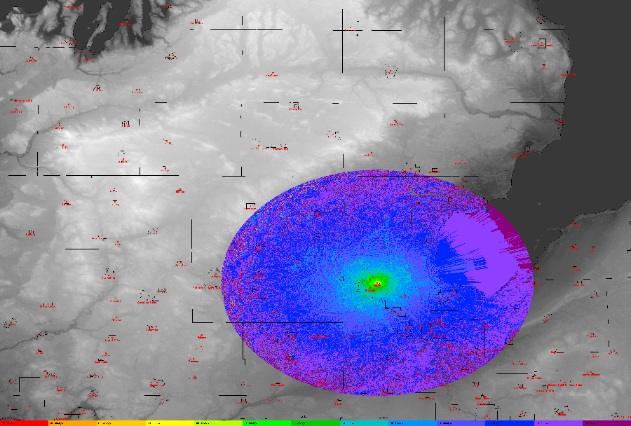
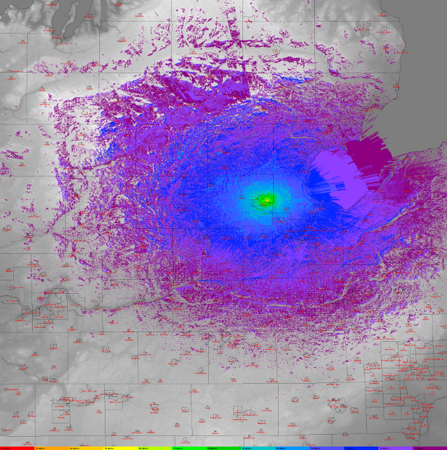
splat is a Surface Path Length And Terrain analysis application which can perform path loss calculations as well as generate coverage maps. Primarily intended for VHF/UHF, it can help plan repeater coverage or plan emergency communications strategies.

⁠5.1.1. Installation and setup

Installing splat is straightforward:

	su -c 'yum install splat'

⁠5.1.1.1. Obtaining Terrain Files

Before it can be useful, splat requires files that describe the terrain around the station to be modelled. First, determine the latitude and longitude of the station. Then download the nine terrain files centered on that latitude and longitude from http://e0srp01u.ecs.nasa.gov/srtm/version2/SRTM3/.

Unzip the nine files and convert them from hgt files to sdf with the srtm2sdf utility. For example:

	  srtm2sdf N41W082.hgt

Do this for each of the nine files. Those files can now be placed in a directory where you wish to store terrain files, or they can be placed in the directory where you wish to work with splat

If you will be modelling stations over a wide geographic area, you may wish to download and convert additional files. splat will select those files it requires for a particular calculation.

⁠5.1.1.2. Obtaining cartographic boundary files

splat will work with just the terrain files. However, for path loss maps, the resulting maps can be more useful if they are marked with political boundaries and names of towns and cities. For the United States, county outlines can be downloaded from http://www.census.gov/geo/www/cob/co2000.html#ascii and 'census designated areas' from http://www.census.gov/geo/www/cob/pl2000.html#ascii.

For each of these, there are two files, an xxyy_d00.dat and xxyy_d00a.dat, where xx is 'co' for county and 'pl' for place, and yy is a state number. A file of place names can be generated from the 'a' file with the citydecoder utility. For example:

	  citydecoder pl37 >cities.dat

The cities.dat file is simply a list of names followed by latitude and longitude. You may edit the file with a text editor to insert additional places which will be marked on the map with a red dot.

⁠5.1.2. Using SPLAT!

splat can perform calculations for a particular path, or generate a map showing path loss or signal strength over a region. In any case splat needs at least one file identifying the transmitter location. For a specific path, it needs an identical file for the receiver. If you would like signal strength calculations, you will need another file with more details about the transmitter.

⁠5.1.2.1. The QTH file

You tell splat about a particular station (transmitter or receiver) with a qth file. This file has four lines:

The name of the station
The latitude of the station
The longitude of the station
The antenna height above ground

Here is an example qth file:

The qth file should be named for the station. The name of the file in the above example would be W8KEA-4.qth.

By default, splat uses British units; heights are in feet, distances are in miles. However, invoking splat with the -metric switch will cause it to use metric units.

⁠5.1.2.2. The LRP file

If you would like splat to calculate signal strengths, it needs to know a little more about the transmitter. You provide this information in a file whose name matches that of the qth file but has an extension of lrp.

The lrp file has 9 lines:

Earth Dielectric Constant. If you do not have measured data available, the splat man page has a table that can help you estimate a value.
Earth Conductivity
Atmospheric Bending Constant
Frequency
Radio Climate. This is a code describing the terrain. See the table in the man page
Polarization
Fraction of situations. This and the following line reflect how the Longley-Rice calculations are to be carried out. In the example below, splat will calculate the maximum path loss experienced 50% of the time in 50% of the situations.
Fraction of time
Effective radiated power - power out less feedline loss times antenna gain

	  15.000  ; Earth Dielectric Constant (Relative permittivity)
	  0.005   ; Earth Conductivity (Siemens per meter)
	  301.000 ; Atmospheric Bending Constant (N-Units)
	  145.090 ; Frequency in MHz (20 MHz to 20 GHz)
	  5       ; Radio Climate
	  1       ; Polarization (0 = Horizontal, 1 = Vertical)
	  0.50    ; Fraction of situations
	  0.50    ; Fraction of time
	  126.00  ; ERP

You may leave out the last line in which case splat will calculate only path loss.

⁠5.1.2.3. Making a map of coverage

⁠

Figure 31. Coverage map with constrained distance

⁠

Figure 32. Coverage map with unconstrained distance

⁠

Figure 33. Signal Strength Legend

⁠5.1.2.4. Calculating a point-to-point path

⁠5.2. xnec2c

xnec2c is a GUI wrapper on the popular NEC2 antenna modeling program. The application allows the design of an arbitrary antenna, and displays gain, impedance and other useful results.

⁠

Figure 34. xnec2c - yagi

xnec2c displays its output in up to three windows. The first window shows the model the user has provided:

⁠

Figure 35. Structure display of a collinear

The user may rotate the view with the two numeric controls. The X, Y and Z buttons permit views along the three axes, and the curved arrow button returns to the default isometric view.

Selecting Radiation Pattern from the View menu opens the radiation pattern window (Figure 36, “Radiation Pattern Display”). The view may be rotated in the same manner as the structure window. Buttons at the top allow for selection of the radiation pattern or the field pattern display.

⁠

Figure 36. Radiation Pattern Display

The dB / MHz controls allow for specifying the precise frequency at which the gain is to be displayed.

Selecting Frequency Plots from the View menu opens the frequency data plots window (Figure 37, “Frequency Data Plots Display”). Buttons along the top permit display of SWR, impedance, phase, etc.

⁠

Figure 37. Frequency Data Plots Display

Clicking on the graph causes the gain, SWR and impedance to be displayed immediately above the graphs for the selected frequency.

More complete documentation is installed with the application and may be found at file:///usr/share/doc/xnec2c-1.5/xnec2c.html after the application has been installed.

⁠5.2.1. Improving calculation performance

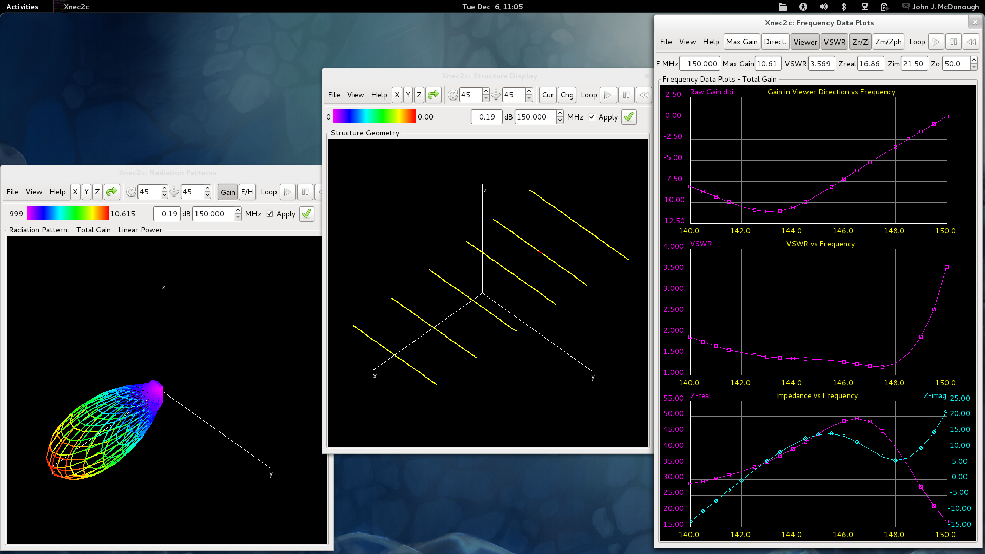
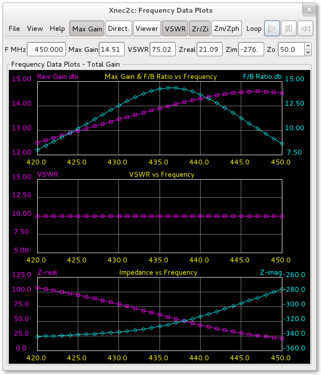
When a complex antenna with many segments and many frequency steps is required, the calculation can take some time. xnec2c is able to take advantage of modern, multicore processors by specifying -j <n>, where <n> is the number of subprocesses to spawn. Many multicore processors can create two threads per core, so a command line entry of

xnec2c -j 8 &

can improve performance by almost a factor of eight on a quad core processor.

⁠6. Packet and APRS

⁠6.1. ax25-tools

⁠6.1.1. Setting up ax25-tools

Before starting ax25-tools you must first edit /etc/ax25/axports to reflect your particular TNC.

⁠

Figure 38. /etc/ax25/axports

The file consists of a single line containing six fields. The fields are described in man axports. The file may also contain comment lines identified by a # character at the beginning of the line.

⁠6.1.2. Starting ax25-tools

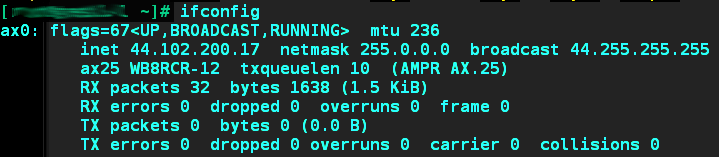
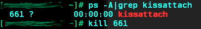
ax25-tools are started with the kissattach command. The arguments required are 1) the port to which your TNC is attached, 2) the name to be given to the port that ax25-tools will attach, and 3) the IP address to be assigned to the interface. The interface names will begin with ax0 and increase as additional TNCs are connected.

⁠

Figure 39. Starting AX25

In the example above, the TNC is attached to /dev/ttyAMA0, the port will be the 145.09 port as described in axports above, and the interface will be assigned the IP address of 44.102.200.17.

As shown above, you will also want to establish one or more routes. As a minimum, you will want to route the 44/8 network (the amateur radio packet network) to your newly created interface. Typically, some node will be designated as a router for your local radio network and you will want to designate that node as your router for 44/8 traffic. Your routes may be different depending on your local resources and your own RF footprint. If there is no router in your area, you may wish to simply route all 44/8 traffic to your ax0 interface.

⁠6.1.3. Using ax25-tools

ax25-tools creates a network interface which may be viewed with ifconfig like any other interface.

⁠

Figure 40. ifconfig

Since the interface has an IP address, it may be used with any application expecting to use an Internet port, assuming, of course, that an appropriate server exists within radio range. Thus, if an IP BBS is nearby, tools such as telnet, ftp, or a web browser may be used.

⁠

Figure 41. Using AX25

Note that the packet connection tends to be quite a bit slower than wired Internet, so the connections will take much longer than you might expect.

ax25-tools only provides the interface. The package ax25-apps (Section 6.2, “ax25-apps”) provides a number of simple AX.25-only applications that may be used in the event that IP packet is not available in your area.

⁠6.1.4. Stopping ax25-tools

ax25-tools is stopped by merely killing the kissattach process. Do this by identifying the PID for the process and killing that process:

⁠

Figure 42. Stopping AX25

⁠6.2. ax25-apps

ax25-apps provides a number of AX.25-only applications for use with ax25-tools in environments where there is no packet IP infrastructure. Of particular interest are axlisten and axcall. These applications can also be used with soundmodem.

⁠6.2.1. axlisten

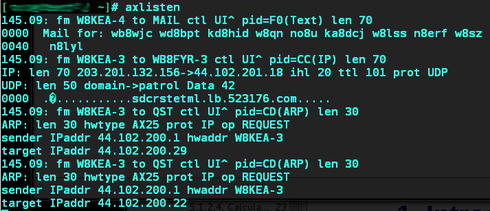
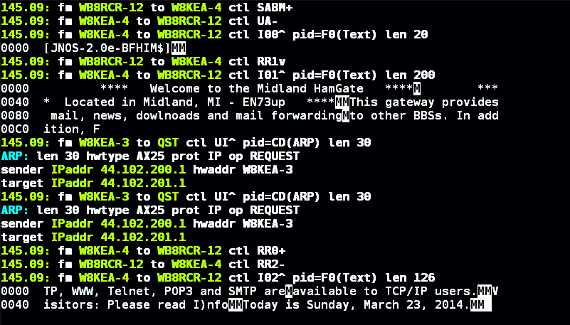
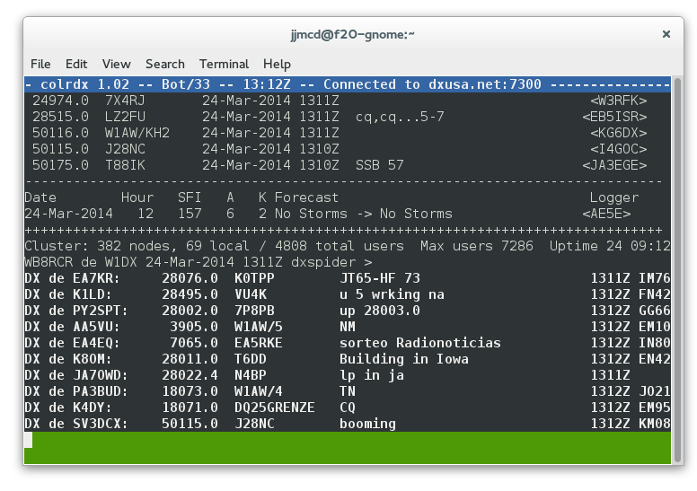
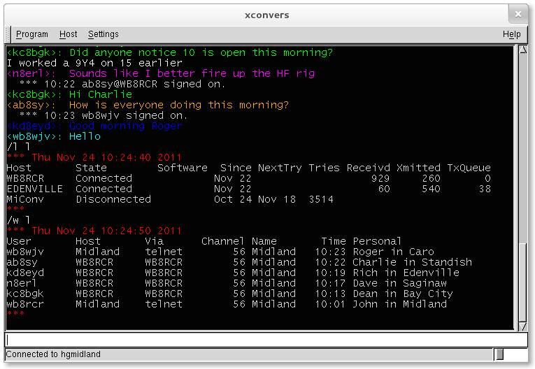
axlisten allows the user to monitor packets on the AX.25 port. If invoked with the -a switch, both incoming and outgoing packets are displayed.

⁠

Figure 43. axlisten

Note that the packets are each identified with the port, and that IP, UDP and ARP packets are also identified.

Should axlisten be started with the -c switch, the screen is cleared and parts of the packets are color coded:

⁠

Figure 44. axlisten

⁠6.2.2. axcall

axcall attempts to make an AX.25 connection to a remote node. Call axcall with the name of the port and the SSID of the node to which you wish to connect.

For several seconds the connection attempt will display:

⁠

Figure 45. axcall, connecting

Once connected, the screen will clear and be divided into two parts. The larger, upper part, displays input from the remote node. The smaller, lower part will accept typing to be sent to the remote node.

⁠

Figure 46. axcall, connected

When the remote node disconnects, the window will be cleared.

⁠6.3. colrdx

colrdx is a simple client for amateur radio DX clusters. In a split-screen display you can type commands for the cluster in the bottom part. Messages from the DX cluster will appear in the main window. There is also a status line at the top with some basic information.

⁠

Figure 47. DX Cluster Client

To start colrdx, open a terminal window and type the command. You must provide your callsign and the name of the packet cluster. Optionally, you may also wish to provide the port:

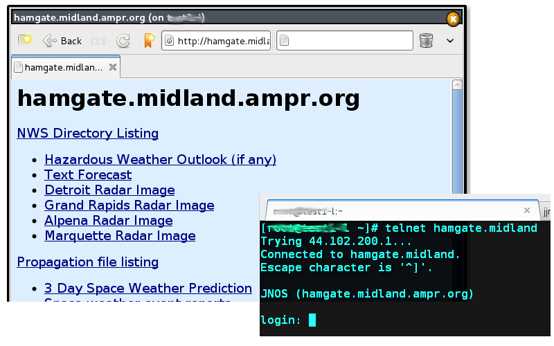
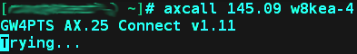
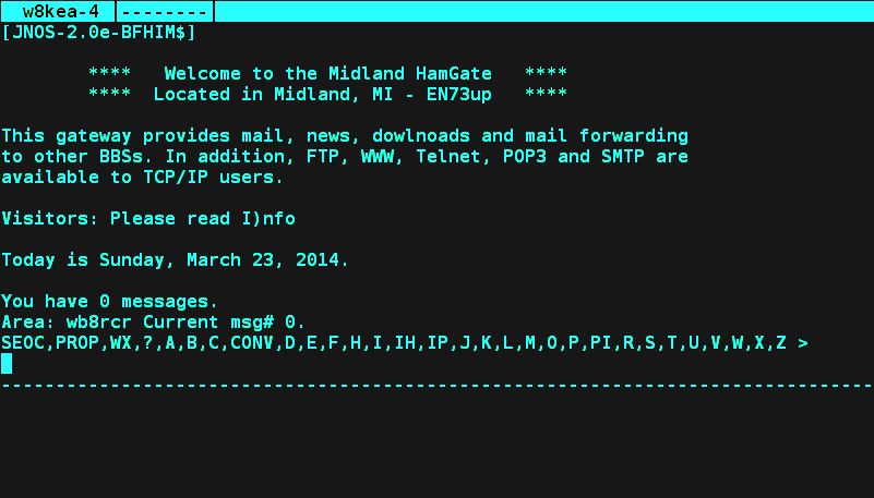
colrdx -c <call> <nodename> [<port>]

You will see some introductory information from the cluster and spots will begin to appear. You may type commands to the cluster (dependent on the particular cluster). To exit type quit.

There is a manpage with additional details.

⁠6.4. soundmodem

soundmodem provides an AX.25 interface through a sound card device, eliminating the need for a TNC.

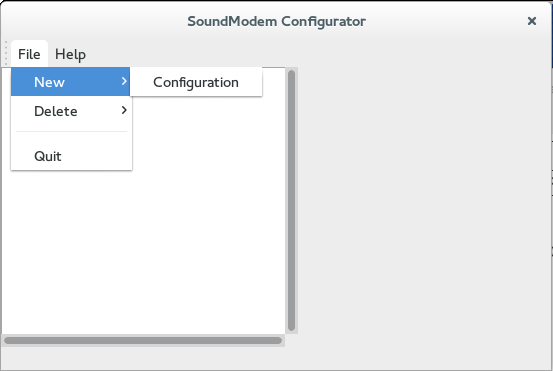
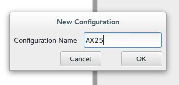
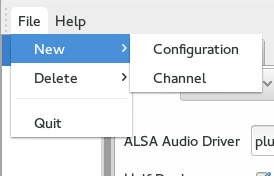
Before it can be used, soundmodem must be configured by issuing the command: soundmodemconfig&. This will launch the configuration dialog.

Multiple configurations can be configured, the first step is to start a new configuration:

⁠

Figure 48. soundmodemconfig

This will open a dialog requesting a name for the configuration:

⁠

Figure 49. Naming the configuration

Enter the appropriate data for your sound card. The lower part of the dialog is only applicable if hamlib is to be used. The Channel Access tab contains a few TNC parameters and generally the defaults should be used until more experience is gained with the particular channel:

⁠

Figure 50. Configuration panel

After creating the configuration, it is now necessary to create a new channel:

⁠

Figure 51. New channel

The channel contains specifics about the modulation as well as identification. For the modulator, the values shown below are typical for VHF packet:

⁠

Figure 52. Modulator configuration

The demodulator will typically be set to the same values as the modulator:

⁠

Figure 53. Demodulator configuration

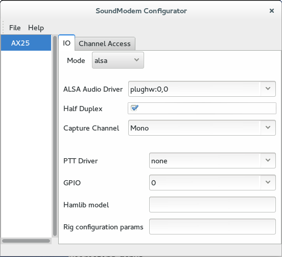
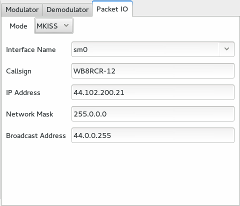
the Packet I/O contains identification specific to your station. The Interface Name must match the name of port in /etc/ax25/axports (Figure 55, “/etc/ax25/axports”) if the ax25-apps (Section 6.2, “ax25-apps”) is to work properly. Similarly, the Callsign, which should contain your station's SSID, must also match the value in axports. The IP Address should be the address assigned by your local AMPRnet coordinator. The remaining fields have their typical meaning.

⁠

Figure 54. Packet I/O configuration

You must also set up /etc/ax25/axports to create a port for your sound device. (Refer to Section 6.1, “ax25-tools”.)

⁠

Figure 55. /etc/ax25/axports

You may now use the axlisten and axcall applications described in Section 6.2, “ax25-apps”. If you have IP resources available, you may also use ordinary network applications. soundmodemconfig provides basic routes, but depending on your local environment, you may wish to add additional routes.

⁠6.5. xconvers

xconvers is a client for packet based CONVerse bridges. When selected, xconvers will present a blank screen. Choosing Open... from the Host will open a dialog allowing the user to enter the name and port of the host.

⁠

Figure 56. Host open dialog

Once connected, the user will see conversation on the channel. User input is seen in the lower part of the window and entered into the CONVerse bridge when Return is pressed.

⁠

Figure 57. xconvers

Input from different users is seen in different colors. The colors and fonts may be adjusted by selecting Preferences... from the Settings menu.

⁠6.6. xastir

xastir is an APRS application that allows users to send and receive position reports, messages, weather data, and other information over packet radio. Data received is displayed on a map allowing the user to get real-time information about a certain area. The user may also fetch trails from findu.com and display them on the map when connected to the Internet.

⁠

Figure 58. xastir

The map may be selected from a large number of sources. Facilities are also provided for drawing fixed items on the map as well as making measurements. The user may make specific queries to weather stations and Igates.

⁠6.6.1. Initial Setup

Select Station from the Configure submenu of the File menu. This will bring up a dialog allowing the user to enter basic station information such as call, location, and symbol to be used.

⁠

Figure 59. Station Setup

Selecting Defaults from the Configure submenu of the File menu will elicit a dialog allowing configuration of some common default information, such as whether the station is mobile or fixed and whether to allow IGate traffic.

⁠

Figure 60. Defaults

Select Interface Control from the Interface menu. Click Add and select an interface type. then click Add. A dialog specific to the interface type will appear. The image below shows a KISS TNC as an example, but the operator may select Internet servers, GPS devices and other interfaces as well.

⁠

Figure 61. Setting up a TNC

Once interfaces are configured, some small symbols will appear in the status bar toward the lower right of the window. The upper semi-circles represent the various interfaces; different types are shown as different colors. The bottom symbol represents the interface status; green for active, empty for inactive, and red for an error. Between these two symbols an arrow will appear briefly whenever data is being transferred.

⁠

Figure 62. Interface Status

⁠6.6.2. Setting up maps

xastir comes configured for a number of online map sources, and the documentation includes pointers to many online map sources. Maps may be vector maps or raster maps, and they may be provided in a number of different formats. In general, maps downloaded and stored locally will be retrieved faster than those retrieved online.

Although raster maps often look better, vector maps typically offer better flexibility and performance. You may select a number of maps and raster maps may be overlaid on other maps. You could, for example, select a satellite image background, overlay it with a vector map of roads, and overlay that with weather radar.

Select Map Chooser from the Map menu. Highlight those maps desired and click Apply to activate the maps.

⁠

Figure 63. Map Chooser

Click Properties on the Map Chooser to activate the Map Properties dialog. This dialog allows you to select the order in which maps will be layered, and whether areas will be filled (when appropriate).

⁠

Figure 64. Setting map layers

Often one would like to return to a particular view. Select Map Display Bookmarks from the Map menu to bring up the Map Bookmark display. The user may then type a name for the current view in the New Name box and click Add on that dialog to save that view. In the future, clicking Activate! from this same dialog will return to the selected view.

⁠

Figure 65. Bookmarks

The user may select a background color from the Background Color submenu of the Configure submenu of the Map menu. Note that raster maps or filled areas will cover the background color.

⁠

Figure 66. Light Background

Notice that if a light color is selected as a background on a vector map, the stations can sometimes be difficult to see.

⁠

Figure 67. Dark Background

But selecting a background too dark makes the map features difficult to identify, while allowing the stations to stand out. A medium color selection will allow the best of both, although certain uses will lend themselves to an emphasis on one or the other.

Select a text style from the Station Text Style submenu of the Configure submenu of the Map menu. By selecting Text On Black stations will stand out better when a light background has been selected.

⁠

Figure 68. Text Properties

⁠6.6.3. Tracking Stations

Select Track Station from the Station menu. A dialog will appear allowing the call of a station to be entered. When this station is seen to move, a track will be drawn on the map showing the station's past positions.

⁠

Figure 69. Tracking a station

If a station which is moving has not been heard from in a while, xastir will use "dead reckoning" to predict where it might be, if dead reckoning has been enabled. Dead reckoning is enabled in the Filter Display submenu of the Station menu. "A while" is configured in the Timing menu item of the Configure submenu of the File menu.

⁠

Figure 70. Dead Reckoning

Historical tracks may also be downloaded from the findu website. Select Fetch Findu Trail from the Station menu.

⁠

Figure 71. Downloading a findu trail

A dialog will appear which allows for the entry of the desired call, as well as two sliders which allow for adjustment of the period for which the trail is desired. It may take some time to download a long trail. The trail will be displayed on the map just as with RF trails.

⁠7. Circuit Design and Simulation

⁠7.1. gEDA

gEDA is a collection of packages for schematic capture, netlist generation, circuit simulation and PCB layout. Included in the geda suite are:

geda-docs - Documentation and example files

geda-gattrib - gEDA attribute editor

geda-gnetlist - Generates a netlist from a gEDA schematic

geda-symbols - A library of symbols for gEDA

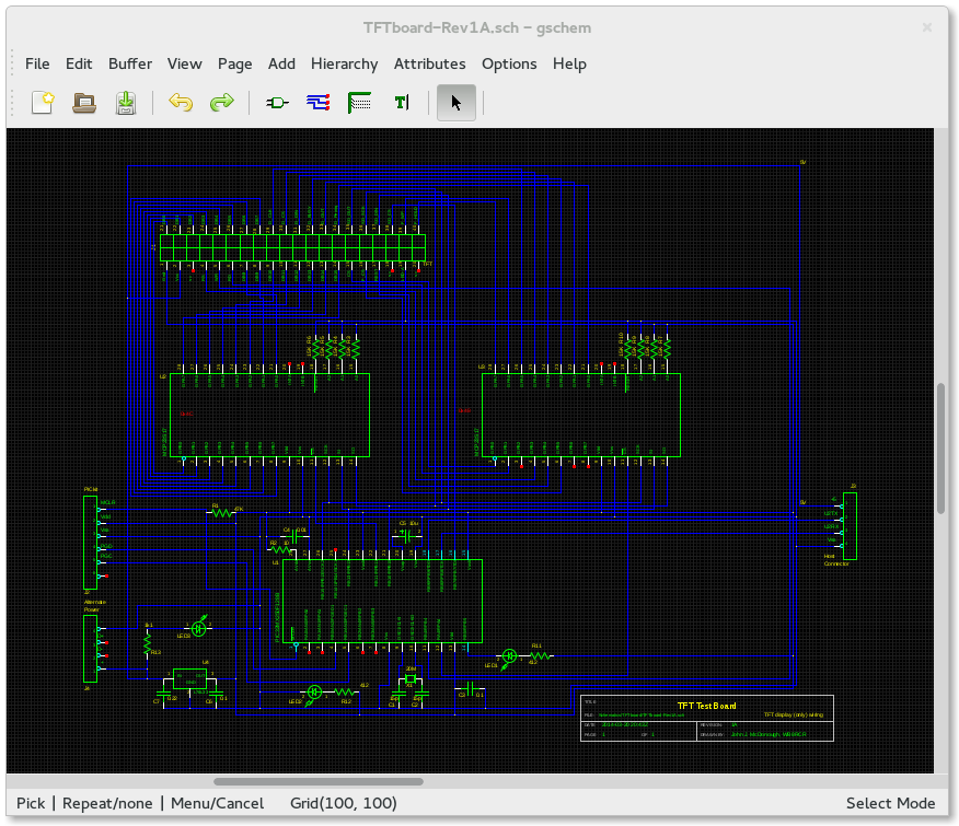
geda-gschem - The gEDA schematic capture application

geda-gsymcheck - A symbol checker for schematics

In addition to the geda-utils utilities package, geda-gaf design automation package, and libgeda the gEDA library.

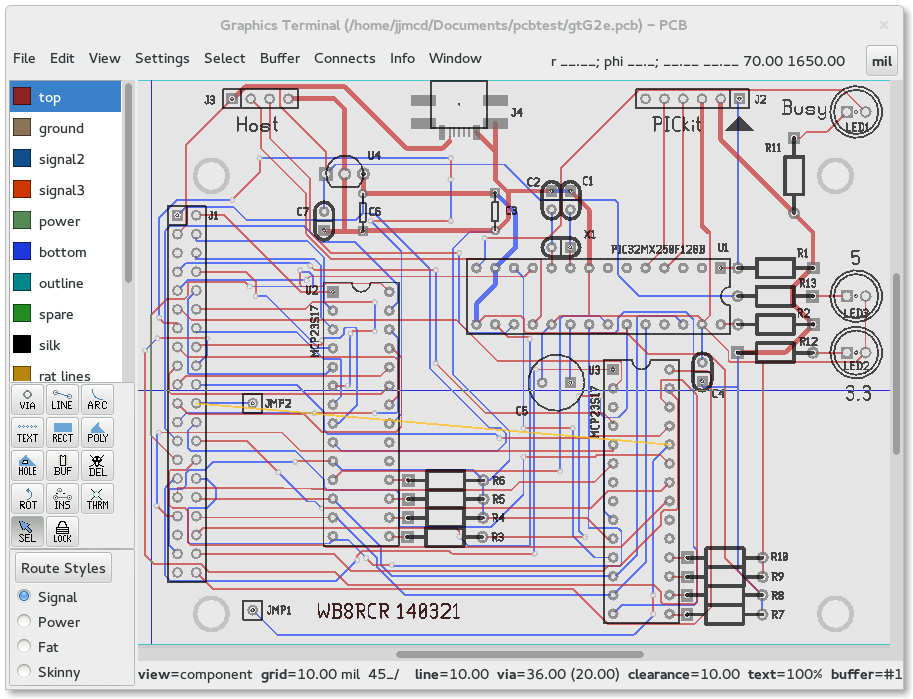
Closely tied into gEDA and mentioned elsewhere in this guide are:

pcb - The printed circuit board layout application

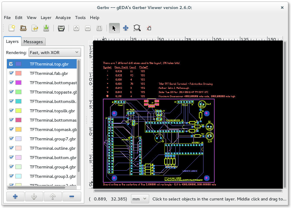
gerbv - Gerber viewer

gwave - The waveform viewer

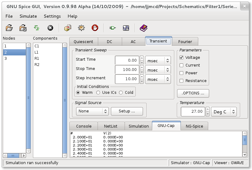
ngspice - The circuit simulator

gspiceui - A GUI interface for ngspice

⁠

Figure 72. geda - gschem

Users wishing to take full advantage of gEDA should consider installing the Electronic Lab group which includes all the above components as well as the electronics-menu package and a number of other useful applications.

⁠7.2. gerbv

grebv is a viewer for Gerber files.

In addition to selectively viewing and coloring Gerber layers, gerbv allows the user to export the image in a number of image formats for publication, as well as RS-274X compliant Gerbers and Excellon drill files.

⁠

Figure 73. gerbv

⁠7.3. pcb

pcb allows for the capture of printed circuit board layouts.

In addition to purely manual layout, pcb can import netlists from gschem. A large number of footprints are available or the user may develop his own.

⁠

Figure 74. pcb

The application can generate a bill of material and drill file, and in addition to printing various layers can export in a number of popular formats.

⁠7.4. gspiceui

gspiceui is a frontend to a SPICE simulation. The user may choose between the gnucap or ng-spice backends.

⁠

Figure 75. gspiceui

gspiceui can open a netlist produced by gnetlist and run the SPICE simulation without having to know the various SPICE commands.

⁠8. Miscellaneous Applications

⁠8.1. CuteCW

CuteCW is a Morse code training program that not only trains the user in decyphering morse code but also provides methods for increasing their comprehension speed. CuteCW will also sound Morse code out of the computer speakers and will read text out as Morse code.

⁠8.1.1. Installing CuteCW

CuteCW is simply installed like most applications:

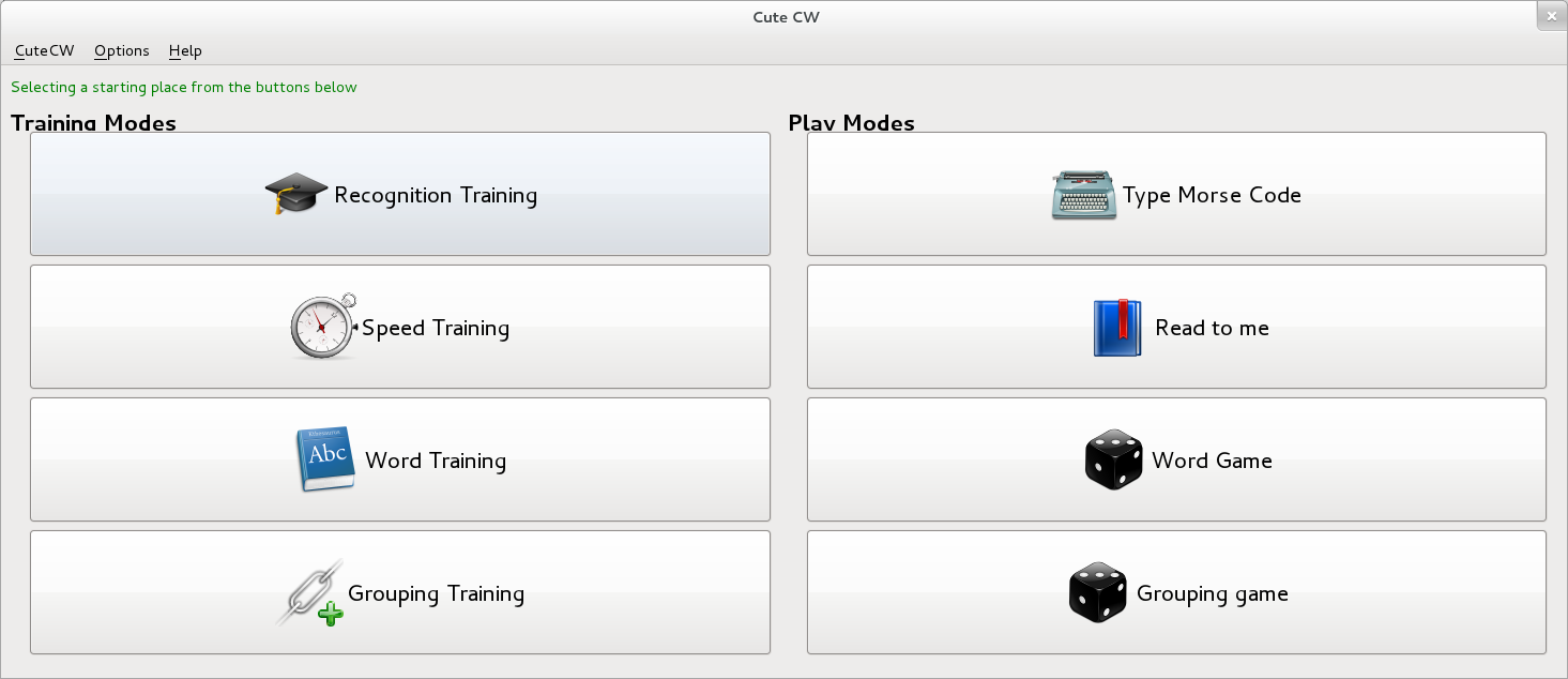
sudo yum install cutecw

⁠8.1.2. Starting CuteCW

CuteCW may be started from the menu by selecting Applications->Education->CuteCW or from the command line by typing cutecw.

⁠8.1.3. Using CuteCW

CuteCW is quite easy to use. Eight choices are given to help with your learning experience.

⁠

Figure 76. CuteCW

In the training mode, CuteCW will help with your recognition of characters, words, and groups. It will also help you increase your speed. In the play mode, CuteCW will read text to you in Morse code, allow you to type out Morse code messages, and even play games.

⁠8.2. dxcc

dxcc is a simple application to give quick information about a DXCC entity. Simply enter the callsign and see the country, WAZ and ITU zones, and other useful information.

⁠

Figure 77. dxcc

⁠8.3. gpredict

gpredict is an application to show the locations of various satellites. Satellite locations and ground footprints are shown on a map, a polar display showing the user's sky view of the spacecraft is available, and another window shows various details of the orbit. The displays are updated in real time.

⁠

Figure 78. gpredict

Before using gpredict, the user should select Preferences from the Edit menu and set up station location and display name. (Refer to Figure 79, “Select Ground Station”.)

⁠

Figure 79. Select Ground Station

First, select the Ground Stations tab and click Add New.

A dialog will pop up (Figure 80, “Ground Station Settings”) which will permit entering the station details. Note that by clicking the Select button, the location may be chosen from a list.

⁠

Figure 80. Ground Station Settings

When complete, be sure to check that the desired station is selected as the Default so it will be displayed on the map (the right column in Figure 79, “Select Ground Station”).

Next, the user should update orbital parameters by selecting Update TLE from the Edit menu. Downloading these values may take a few moments.

By default, a few amateur satellites are shown. The lower portion of the display will show details for the spacecraft currently in view. Orbital parameters for another satellite may be selected from the dropdown to the left of the satellite name.

There are a number of other displays available, and additional groups of satellites may be configured which may be shown in tabs (File -> New module). Clicking on the small downward triangle to the right of the window (Figure 81, “Module Menu”) brings up a menu which permits editing an existing module.

⁠

Figure 81. Module Menu

Also available from that module menu is a Sky at a glance selection which brings up Figure 82, “Sky at a glance”, showing which spacecraft in the module will come into view within the next eight hours.

⁠

Figure 82. Sky at a glance

In the map view, hovering over a spacecraft will display the current position information:

⁠

Figure 83. Position Display

⁠8.4. gresistor

gresistor is a simple application for decoding resistor color codes. Select the number of bands on the resistor and each of the colors of the bands, and the resistor value and tolerance are displayed.

⁠

Figure 84. gresistor

⁠8.5. ibp

ibp is a simple application that shows beacons which are part of the International Beacon Project. A number of beacons around the world transmit at predetermined times. The ibp application shows you which beacons are currently transmitting.

⁠8.5.1. Installing ibp

ibp is simply installed like most applications:

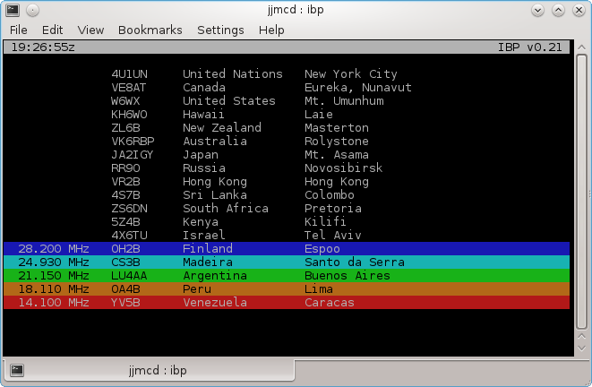
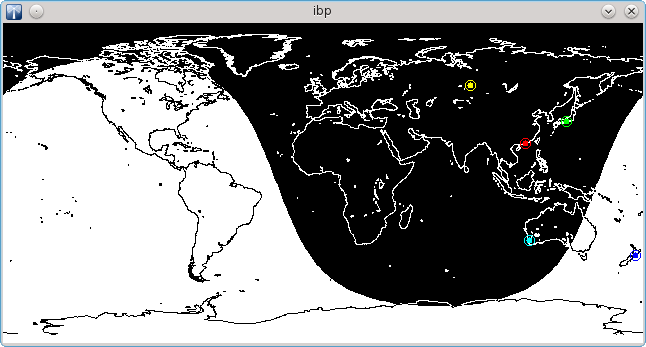
sudo yum install ibp

No additional configuration is required, however, ibp expects that the time on the system is correct. Synchronizing your system with one of the many timeservers is recommended.

⁠8.5.2. Starting ibp

ibp may be started from the menu by selecting Applications->Other->ibp or from the command line by typing ibp.

When ibp is started, by default, two windows will open. The first is a simple text screen showing a list of beacons with the currently transmitting beacons highlighted:

⁠

Figure 85. ibp - text screen

The second window shows a map of the world with a colored dot for each transmitting beacon:

⁠

Figure 86. ibp - map

There are a number of arguments you may specify to affect how ibp behaves when it is started from the command line:

-c, --nocolor - causes the text window to be displayed only in monochrome. The graph window is still in color.
-m, --morse - In single beacon mode, causes the callsign of the transmitting beacon to be displayed at the bottom of the text window in Morse.
-x, --nograph - Don't display the map window.

⁠8.5.3. Running ibp

While ibp is running, the highlighted lines on the text display and the dots on the map will periodically change as different beacons take on the transmitting task.

There are several commands you can enter into the text screen to affect the behavior of ibp:

digits 1 through 5 - causes only one band to be displayed. Since one is normally only monitoring a single band at a time this can lead to faster identification of the beacon of interest. This is also useful for visually challenged operators.
M - toggles between single band and multi band mode. If a single band was displayed, typing M will cause all five bands to be displayed. If five bands were displayed, the previously selected single band will be displayed.
Q - causes ibp to exit.

⁠8.6. rcrpanel

rcrpanel is a command line application wich allows layout of panels for electronic equipment. rcrpanel accepts as input a text file describing the panel. It produces as output a Postscript stream of an image of the panel. The Postscript stream may be redirected to a file, a Postscript printer, or piped to another application such as Ghostscript.

By taking a text description of the panel, rcrpanel allows precise placement of controls and annotation, which can be difficult to achieve with a GUI interface. rcrpanel provides scripting elements for text, controls of various sizes, and even calibrated dials.

⁠

Figure 87. Example Panel

⁠8.6.1. Running rcrpanel

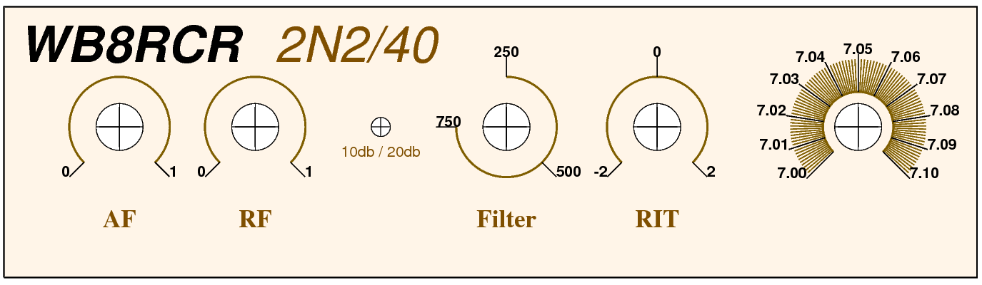
rcrpanel accepts a single command line parameter, the input file containing the description of the panel. It produces its output on stdout, which means that in most cases, the user will redirect the output to a file. For example:

rcrpanel mypanel.txt >mypanel.ps

There are no command line switches available.

The output image will be centered on a standard size page. The smallest page on which the panel will fit is selected from the following list, in order:

216x179 mm - U.S. Letter

210x297 mm - A4

216x279 mm - U.S. Legal

297x420 mm - A3

279x432 mm - Tabloid

594x841 mm - A1

559x894 mm - D

841x1189 mm - A0

1000X1414 mm - B0

⁠8.6.2. The Input File

The input file contains lines describing the various controls. Most lines are of the form

Command = something

where the spaces around the equal sign are significant, and the command itself is case-sensitive.

Measurements are in units of millimeters. Angles are in degrees. Colors are given as 24 bit C style integers where each byte represents the amount of red, green, or blue.

In general, the order of commands makes no difference. However, the Text command must be immediately followed by a line containing the text to be displayed, and those commands affecting the appearance of a Dial affect the preceding Dial command.

⁠8.6.2.1. Background

This command takes a single color following the equal sign. The entire panel will be filled with this color.

Background = 0xfff5e8

Note, however, that the interior of controls will not be filled with this color, allowing the alignment marks to be viewed for drilling, even if the panel were filled with a dark color.

⁠

Figure 88. ControlPhone on a dark background

⁠8.6.2.2. ControlLarge

This is used for large diameter controls such as large pots and the like. It takes 2 values after the equal sign representing the position of the control on the panel.

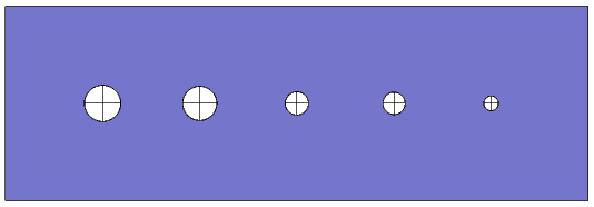
ControlLarge = 23.0 30.0

⁠8.6.2.3. ControlLED

This command generates an outline for a 5 mm LED. Like the other control commands, it takes 2 values, the X and Y positions on the panel of the center of the LED.

⁠8.6.2.4. ControlPhone

This is used for 1/4" phone jacks and similar controls. The 2 values after the equal sign represent the position on the panel.

⁠8.6.2.5. ControlSmall

This command generates an outline for a 3.5 mm phone jack. The two values are the X and Y positions of the jack on the panel.

⁠8.6.2.6. ControlTiny

This command generates an outline for a 2.5 mm phone jack. The two values are the X and Y positions of the jack on the panel.

ControlTiny = 75.0 30.0

⁠

Figure 89. Large, Phone, LED, Small and Tiny controls

⁠8.6.2.7. Panel

This command defines the size of the panel. The 2 dimensions are the width and height of the panel.

Panel = 193.675 53.975

⁠8.6.2.8. Reverse

This command takes no arguments. If this command appears anywhere in the input file, the resulting PostScript will be flipped left to right (for printing on the reverse side of transfer media or transparency material).

⁠8.6.2.9. Text

This command is somewhat different from the others. After the equal sign, it takes 3 floating point numbers, a color, and a text string. The first 2 floating point numbers are the X, Y position of the text on the panel. The third number is the height of the text. The color represents the color of the text, and the text string represents the font to be used. No checking is done before preparing the PostScript; you are responsible for ensuring that the font is available on your printer.

This command is then followed by another line containing the text to be displayed.

Text = 100.0 10.0 5.0 0x7f4f00 Times-Roman-Bold
Filter

⁠8.6.2.10. Dial

This command introduces a new dial. The Dial command describes the X,Y center of the dial. The following commands then further refine the details of this particular dial. This relationship between the Dial command and it's successors is the only place where the order of the commands within the file matters.

Dial = 170.0 30.0

⁠8.6.2.11. Radius

This command takes a single value which is the radius of the circle which forms the inside of the tick marks. This command refers to the current Dial command.

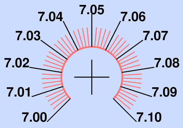
Radius = 7.0

⁠8.6.2.12. Span

This command describes the angle over which the control may operate. Typically, this would be 270 for a potentiometer and 180 for a variable capacitor. This command refers to the current Dial command.

⁠8.6.2.13. NumTicks

This command describes the total number of tick marks, large and small, to be drawn. This is usually an odd number since the starting and ending values are counted. Typically this will be 11, 101, or a similar number. This command refers to the current Dial command.

NumTicks = 101

⁠8.6.2.14. BigPer

This command tells the program how many small tick marks there are per large tick mark. This command refers to the current Dial command.

BigPer = 10

⁠8.6.2.15. SizeTicks

This command describes the length of the small tick marks. This command refers to the current Dial command.

SizeTicks = 6.5

⁠8.6.2.16. SizeBig

This command describes the length of the large tick marks. This command refers to the current Dial command.

SizeBig = 7.5

⁠8.6.2.17. StartingIndicator

This command describes the value to be placed on the furthest counterclockwise large tick mark. This command refers to the current Dial command.

⁠8.6.2.18. IncrementPerBigTick

This command tells rcrpanel how much to increment the value in StartingIndicator for each succeeding large tick mark. This command refers to the current Dial command.

⁠8.6.2.19. SizeFont

This command describes how large to make the annotation on the ticks. This command refers to the current Dial command.

⁠8.6.2.20. ColorCircle

This command takes a single color as an argument, which is used to draw the inner circle. This command refers to the current Dial command.

⁠8.6.2.21. ColorTickMarks

This command permits setting the color to draw the small tick marks. This command refers to the current Dial command.

⁠8.6.2.22. ColorBigTickMarks

This command permits setting the color to draw the large tick marks. This command refers to the current Dial command.

⁠8.6.2.23. ColorText

This command accepts a single color which will be used for the annotation. This command refers to the current Dial command.

⁠8.6.2.24. StartAngle

By default, rcrpanel arranges dials so the dead spot on the control is straight down. This is the desired behavior in almost all cases. However, sometimes you may want to rotate a control to some other orientation. The single argument to StartAngle is the number of degrees clockwise to rotate the control. This command refers to the current Dial command.

⁠8.6.3. Example Dials

⁠8.6.3.1. Frequency Markings for a VCO

Dial = 25.0 25.0
Radius = 7.0
SizeTicks = 4.5
ColorTickMarks = 0xff7777
SizeBig = 7.5
ColorBigTickMarks = 0x000000
StartingIndicator = 7.0
IncrementPerBigTick = 0.01
NumTicks = 51
BigPer = 5
ColorCircle = 0xff7777
SizeFont = 3.0

⁠

Figure 90. 40 meter dial, 270 degrees

⁠8.6.3.2. Markings for a volume control

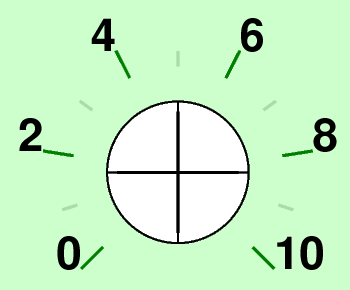
ControlLarge = 25.0 25.0
Dial = 25.0 25.0
Radius = 7.0
SizeTicks = 1.0
ColorTickMarks = 0xaaddaa
SizeBig = 2.0
ColorBigTickMarks = 0x007f00
StartingIndicator = 0
IncrementPerBigTick = 2
NumTicks = 11
BigPer = 2
ColorCircle = 0xccffcc
SizeFont = 3.0

⁠

Figure 91. Volume Control

⁠8.6.3.3. Markings for a VFO (capacitor based)

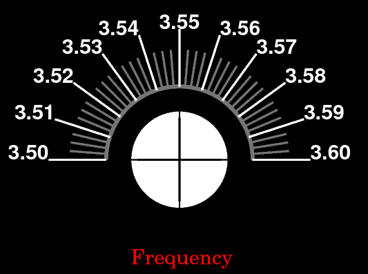
ControlLarge = 25.0 25.0
Dial = 25.0 25.0
Radius = 7.0
SizeTicks = 3.5
ColorTickMarks = 0x777777
SizeBig = 5.5
ColorBigTickMarks = 0xffffff
StartingIndicator = 3.5
IncrementPerBigTick = 0.01
NumTicks = 41
BigPer = 4
ColorCircle = 0x777777
SizeFont = 2.0
ColorText = 0xffffff
Span = 180.0
Text = 25.0 15.0 2.0 0xff0000 Century-Schoolbook
Frequency

⁠

Figure 92. 80 meter VFO

⁠8.7. xgridloc

xgridloc is an application which will translate a latitude/longitude into a Maidenhead grid square. It will also calculate the Great Circle distance and bearing between two locations.

⁠8.7.1. Installing xgridloc

xgridloc is installed like most applications in Fedora:

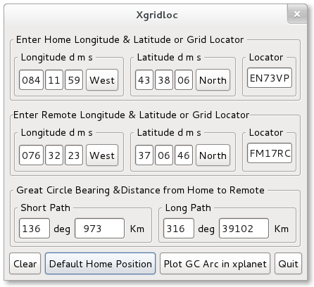
	sudo yum install xgridloc

⁠8.7.2. Setting up xgridloc

xgridloc uses a small configuration file, ~/.xgridlocrc. Before using xgridloc you should replace the default location in the file with your station location using your favorite text editor:

	######### Runtime config file for 'xgridloc' #########
	#
	### Blank lines and those starting with a # are ignored ###
	#
	# The 'Home' location's position.
	# (East Longitude and North Latitude)
	# Format is "East/ddd:mm:ss North/dd:mm:ss"
	West/084:11:59 North/43:38:06
	#
	# The name of the 'Home' location
	Midland
	#

⁠8.7.3. Using xgridloc

xgridloc may be started by selecting item xgridloc icon (usually found in the Internet group) or by issuing the xgridloc command from the command line.

Clicking the Default Home Position button will cause the top location to be filled in with the location you specified in the configuration file.

If you enter a latitude and longitude in either the "Home" or "Remote" location and press Enter, the corresponding Locator box will be filled in with the Maidenhead grid square for that location.

⁠

Figure 93. xgridloc

If both locations are filled, the Great Circle bearing and distance will appear at the bottom of the window.

⁠8.8. xwota

xwota allows for monitoring and querying the WOTA database. It operates much like a DX Cluster client, except it uses the database rather than a cluster. Refer to http://www.wotadb.org for information about the WOTA database.

Selecting Connect from the Xwota menu will connect to the database. New reports will appear on the screen as they arrive.

⁠

Figure 94. Who is on the air

The user may also query the database by selecting Query from the Show menu. A dialog will appear allowing the user to enter specific location, frequency, and/or call to be searched for. Clicking Send will then cause the results to be returned at the bottom of the main window.

⁠

Figure 95. Xwota query window

The user may also enter his own report. Before doing this, station information should be entered by selecting Station Info from the Settings menu and filling in the dialog:

⁠

Figure 96. Station Info window

The user may then enter the frequency and optionally a comment in the main window, and click the Update button to cause the report to be sent to the database.

⁠A. Installing Software on Fedora

There are basically two ways to install software from the Fedora repositories; from the GUI using PackageKit and from the command line using yum. Because the yum approach is simpler, throughout this document we describe that method. However, there are a number of details with respect to yum that are useful to know, and some users feel more comfortable with a graphical user interface. Hence, this appendix.

⁠A.1. Installing Software with the GUI

Launch the PackageKit application by selecting the Add/Remove Software icon from the System Tools group.

⁠

Figure A.1. Add/Remove Software

There may be a delay before the controls on the window that appears may be used. This delay may be brief or lengthy, depending on what you have done earlier. The data used by PackageKit is cached, and if it is stale, new data will be downloaded, which may take several minutes.

Type in the name of the package you wish to install in the text box at the upper left, and select the Find button. There may be a delay, and you may need to click the Find button a second time.

The package (perhaps with several others) will appear to the right. The closed box indicates that the package is not installed on your system.

⁠

Figure A.2. Searching for Software

Click on the check box next to the package you wish to install. A blue plus sign will appear over the box indicating that is has been selected to install.

⁠

Figure A.3. Selecting a package to install

You may repeat the process if you wish to install additional packages. When you have selected the packages you wish, click the Apply button at the lower right to install the packages.

Depending on how your system has been configured, you may be prompted to enter the password for the administrative user. If the package is unsigned, or is from a repository you have not used before, you may be prompted for this password again. As a general rule, only administrators may install software.

⁠

Figure A.4. Authorizing the installation

Enter the root password and click Authenticate.

The package will then be installed. When the installation is complete, the package will be shown as an open box, indicating that the package is installed. For some applications, the application's icon may be displayed instead of the open box. The Apply button will be disabled, indicating that there are no pending actions to apply.

⁠

Figure A.5. Package is installed

The Find button searches not only the name of the package, but also the package description. Some common words may reveal several packages, some perhaps not those intended. For example, if you typed in "circuit" with the intent of finding circuit design applications, you may also find applications referring to wired communications circuits as well as racing circuits!

⁠

Figure A.6. Searching the description

Sometimes you may want to try several variations of a word or phrase. If, for example, you are looking for an SSTV application, trying "slowscan" or "slow scan" will fail:

⁠

Figure A.7. Searching the description - failure

The developer of the slow scan application used the word "slow-scan" in his description. PackageKit is not smart enough to guess what you meant or what the original developer was thinking.

⁠

Figure A.8. Searching the description - success

⁠A.2. Installing Software with yum

Unlike PackageKit, where the system administrator may choose to allow non-administrative users to install software, yum requires administrator authentication. There are three ways this can be done:

You may switch to the root user with the su command:
```
[jjmcd@Cimbaoth ~]$ su -
Password: 
[root@Cimbaoth ~]# yum install xastir
Loaded plugins: presto, refresh-packagekit
  ...
```
This is the least desirable method. You must enter the root password, and you can easily forget that you are operating as root. As the root user you can do unlimited damage.
You may use the su command with the -c switch. This allows you to enter the single yum command as root, but immediately switches back to your normal user:
```
[jjmcd@Cimbaoth ~]$ su - 'yum install fldigi'
Password: 
Loaded plugins: presto, refresh-packagekit
  ...
```
Notice that you must surround the command with quotation marks or apostrophes. This still requires you to type the password, and is somewhat more annoying to type, but does not leave you as root ready to do damage.
If the administrator has set you up in the sudoers file, you may use the sudo command:
```
[jjmcd@Cimbaoth ~]$ sudo yum install wxapt
Loaded plugins: presto, refresh-packagekit
  ...
```
This has several advantages; you don't need to type the password, you are not left in a dangerous position, and if desired, the administrator can limit you to a select set of commands so you do not inadvertently cause damage.
Because this is the preferred approach, the examples in this guide use this method. However, it does require setup ahead of time.

yum may determine that additional packages must be installed. yum will list these packages and calculate the total size of the download. It will then ask you whether you want to actually download and install this package or group of packages:

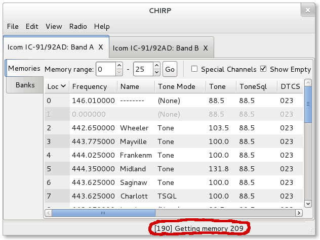
[jjmcd@Cimbaoth ~]$ sudo yum install trustedqsl
Loaded plugins: presto, refresh-packagekit
Setting up and reading Presto delta metadata
Setting up Install Process
Resolving Dependencies
--> Running transaction check
---> Package trustedqsl.i386 0:1.11-3.fc10 set to be updated
--> Processing Dependency: tqsllib >= 1.2 for package: trustedqsl-1.11-3.fc10.i386
--> Processing Dependency: libtqsllib.so.1 for package: trustedqsl-1.11-3.fc10.i386
--> Running transaction check
---> Package tqsllib.i386 0:2.0-5.fc10 set to be updated
--> Finished Dependency Resolution

Dependencies Resolved

================================================================================
 Package             Arch          Version               Repository        Size
================================================================================
Installing:
 trustedqsl          i386          1.11-3.fc10           updates          557 k
Installing for dependencies:
 tqsllib             i386          2.0-5.fc10            updates          167 k

Transaction Summary
================================================================================
Install      2 Package(s)         
Update       0 Package(s)         
Remove       0 Package(s)         

Total download size: 723 k
Is this ok [y/N]:

Answer y or N depending on whether you want to download and install the group of packages.

⁠A.2.1. Searching for Software

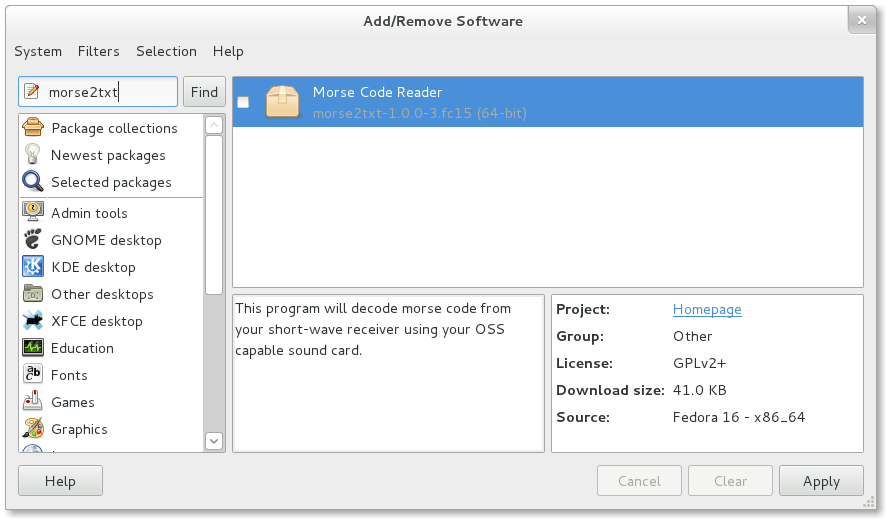
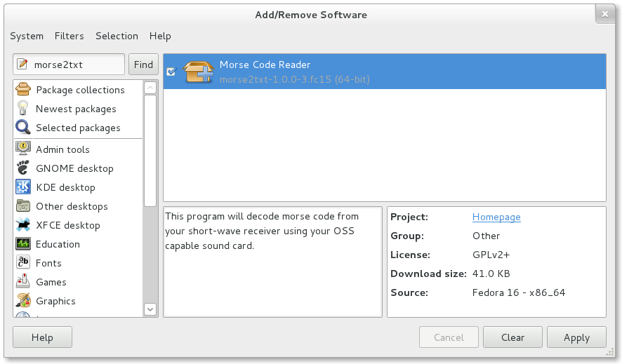
yum gives you a number of choices for locating software you desire. To find information about a package you do not need to provide credentials. Any user may look up information about a package. You may search for specific words in the description using yum search:

[jjmcd@Cimbaoth ~]$ yum search APRS
Loaded plugins: presto, refresh-packagekit
Setting up and reading Presto delta metadata
================================ Matched: APRS =================================
aprsd.i386 : Internet gateway and client access to amateur radio APRS packet
           : data
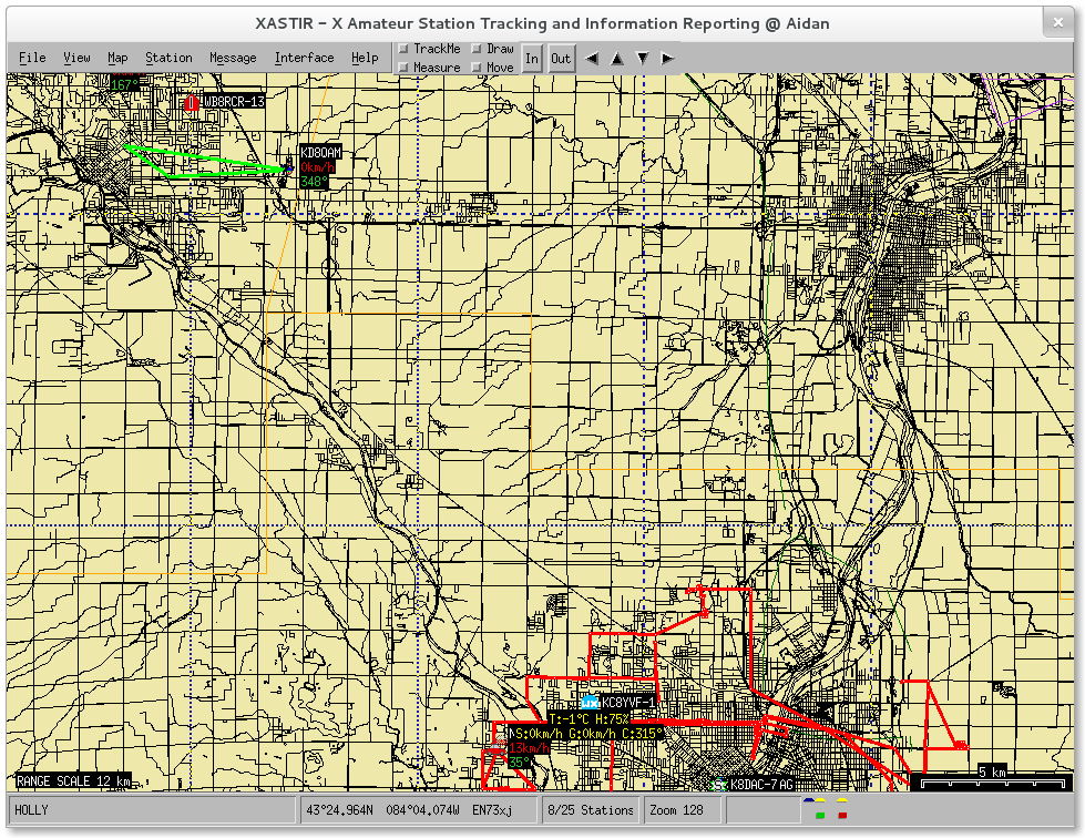
xastir.i386 : Amateur Station Tracking and Reporting system for amateur radio
[jjmcd@Cimbaoth ~]$

yum will return the names of any package with the specified phrase in its description, and a short description. You may get a more detailed description of the package with the yum info command:

[jjmcd@Cimbaoth ~]$ yum info xastir
Loaded plugins: presto, refresh-packagekit
Setting up and reading Presto delta metadata
Installed Packages
Name       : xastir
Arch       : i386
Version    : 1.9.4
Release    : 5.fc10
Size       : 4.0 M
Repo       : installed
Summary    : Amateur Station Tracking and Reporting system for amateur radio
URL        : http://www.xastir.org
License    : GPLv2+
Description: Xastir is a graphical application that interfaces HAM radio
           : and internet access to realtime mapping software.
           : 
           : Install XASTIR if you are interested in APRS(tm) and HAM radio
           : software.

[jjmcd@Cimbaoth ~]$

Notice that yum also tells you whether the package is installed. Yum also gives you the address of the upstream website so you may learn more about the package before installing it.

⁠B. Revision History

Revision History

Revision 19-1

August 21, 2013

Eric Christensen

Branched for Fedora 19

Added CHIRP.

Revision 16.1

January 3, 2012

John McDonough

Added fldigi back in now that it is working

Revision 16.0

December 10, 2011

John McDonough

Changes for Fedora 16:

- New screenshots for F16

- Remove fldigi (not working on 16 yet)

- Updates to installation procedures

- Remove references to old GNOME menu

- Add documentation for xnec2c

- Add documentation fr gspiceui

- Add documentation for gpredict

- Correct error in xgridloc documentation

- Add documentation for gerbv

- Add documentation for pcb

- Other mostly minor touch-ups

Revision 15.90

November 23, 2011

John McDonough

Remove xdx, obsoleted in Fedora 16

Documentation for Chirp

Revision 0.9

November 9, 2010

John McDonough

Documentation for dxcc

Documentation for gresistor

Documentation for callgit

Correct typo in colrdx

Correct typos in xwota

Revision 0.8

November 7, 2010

John McDonough

Documentation for rcrpanel

Documentation for colrdx

Documentation for xconvers

Documentation for xdx

Documentation for xastir

Documentation for gEDA

Documentation for gerbv

Documentation for pcb

Documentation for xwota

Revision 0.7

November 20, 2009

John McDonough

Installing Software appendix

Revision 0.7

October 31, 2009

Eric Christensen

Added xlog installation and setup procedures.

Revision 0.6

October 29, 2009

John McDonough

ibp

Revision 0.5

October 29, 2009

Randy Berry

cwirc

Revision 0.4

October 28, 2009

Eric Christensen

xlog screenshot

Additional info on fldigi

Revision 0.3

October 6, 2009

John McDonough

xgridloc

Revision 0.2

October 4, 2009

John McDonough

Beginning of SPLAT! instructions

Revision 0.1

October 1, 2009

John McDonough

Document skeleton